Conditional Formats: Icon Sets

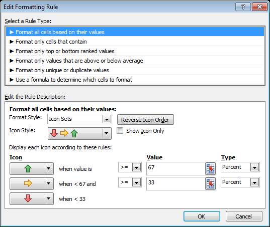
Icon Sets in Excel 2010 make it very easy to visualize values in a range of cells. Each icon represents a range of values. To add an icon set, execute the following steps. 1. Select a range. 2. On the Home tab, click Conditional Formatting, Icon Sets, and click a subtype. Result: Explanation: by default, for 3 icons, Excel calculates the 67th percent and 33th percent. 67th percent = min + 0.67 * (max-min) = 2 + 0.67 * (95-2) = 64.31. 33th percent = min + 0.33 * (max-min) = 2 + 0.33 * (95-2) = 32.69. A green arrow will show for values equal to or greater than 64.31. A yellow arrow will show for values less than 64.31 and equal to or greater than 32.69. A red arrow will show for values less than 32.69. 3. Change the values. Result. Excel updates the icon set automatically. Read on to further customize this icon set. 4. Select the range A1:A10. 5. On the Home tab, click Conditional Formatting, Manage Rules. 6. Click Edit rule. Excel launches the Edit Formatting Rule dialog box. Here you can further customize your icon set (Icon Style, Reverse Icon Order, Show Icon Only, Icon, Value, Type, etc). Note: to directly launch this dialog box for new rules, at step 2, click More Rules. 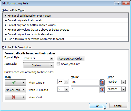7. Select 3 symbols (Uncircled) from the Icon Style drop-down list. Select No Cell Icon from the second Icon drop-down list. Change the Types to Number and change the Values to 100 and 0. Select the greater than symbol (>) next to the value 0. 8. Click OK twice. 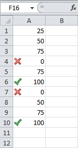Result.